Day_78 01. 모델 경량화 기법 101 - NLP Part 1

모델 경량화 기법 101 - NLP Part 1

1. Overview

1.1 강의 목표

어떤 경량화를 적용해야할까?

• 주어진 환경에 따라 적용할 수 있는 방향이 달라짐
  • Deply 환경(CPU/GPU?, Quantization 적용 시 가속이 가능한 device?)
  • 주된 문제 상황(Latency 를 줄여야한다 // Mobile device 여서 Model size 를 줄여야한다)
  • 경량화 요구 정도(성능 drop 을 감수한 경량화 / 성능 drop 은 절대 없어야한다)
  • HW 리소스(From scrach 로 재학습이 가능한가?)

논문은 각자의 novelty 를 위해, 다른 기법과의 조합을 잘 언급하지는 않는 경향

각 기법의 효과를 알고, 상황의 요구사항에 맞게 어떤 경량화 기법들을 조합해야 할지 판단

각 기법의 주된 특징과, 주요 흐름을 파악!

CV 경량화와 NLP 경량화의 차이점?

• Original task $\rightarrow$ Target task 로의 fine tuning 하는 방식이 주된 흐름
• 기본적으로 transformer 구조(CV 대비 구조의 작은 변화)

Pros:

• Large model $\rightarrow$ small model 방식의 KD 와 좋은 궁합
• 모델 구조가 거의 유사해서, 논문의 재현 가능성이 높고, 코드 재사용성도 높음
  • (e.g. CV 의 경우 VGG $\rightarrow$ Efficientnet 결과가 완전 다르다던지 … 모델 구조로 Cherry picking 을 하는 경우도, …, 모델 구조따라 적용 불가능한 알고리즘도…)

Cons:

• Resource, Resource, …(오랜 학습으로 인한 검증 시간 부족, From scratch 학습에 큰 부담)

1.2 모델 경량화 recap

주요 경량화 기법

• 효율적인 Architecture(MobileNet, EfficientNet 등 + NAS)
• Pruning(Structured/Unstructured)
• Knowledge Distillation(Response based, Feature based, …)
• Weight Factorization(Tucker Decomp, …)
• Quantization

1.3 BERT Profiling

Transformer Encoder 컴포넌트 recap

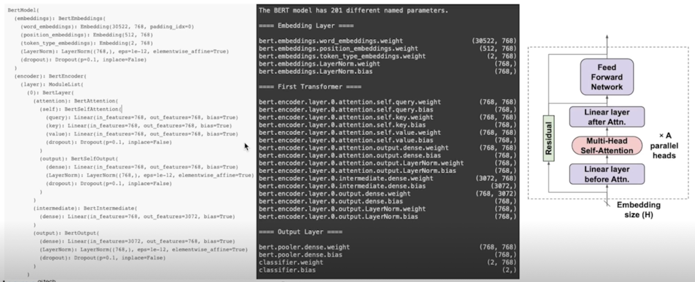
Profiling; Model size and computations

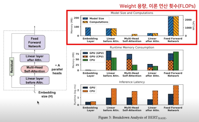
• Embedding layer: look up table 이므로, FLOPs 는 없음
• Linear before Attn: k, q, v mat 연슨으로 after 대비 3배
• MHA: matmul, softmax 등의 연산, 별도 파라미터는 없음
• FFN: 가장 많은 파라미터, 연산 횟수

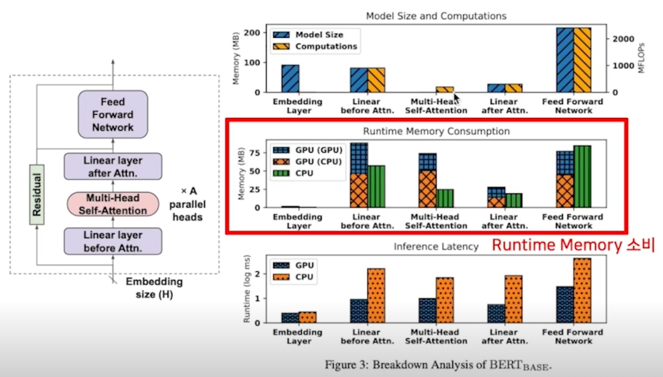
• 효율적인 GPU 연산을 위해 단독으로 CPU 에서 사용하는 메모리보다 소비량이 더 큼(CPU, GPU 에 동일 텐서를 들고있거나 등등)

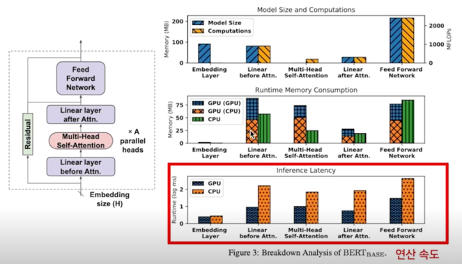
• MHA 파트는 이론 연산 횟수 대비 속도가 매우 느린데, 이는 여러 연산의 조합(matmul, softmax) 때문인 것으로 보여짐
• Linear Layer 에서는 GPU 가 빠른 속도를 보여주나, CPU 는 이론 연산 횟수와 유사한 경향을 보임
• GPU: 57.1ms, CPU: 750.9ms
• FFN 파트가 모델의 주된 bottleneck

2. Paper Review

2.1 Pruning

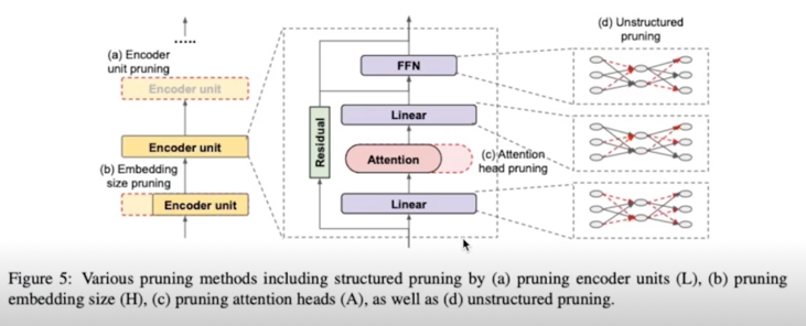
Overview

• Structured: encoder unit(inself), embedding size, attention head
  • 그룹단위로 Pruning 을 하는 것
  • encoder unit 을 하나 없앤다던지 12개 중 하나를 날려버린다던지
  • embedding size 를 줄인다던지
  • attention head 의 개수를 줄인다던지
• Unstructured: sparsify each weight matrix
  • weight matrix 에서 구멍을 뚫는것처럼 sparse 하게 만드는 것

2.1 Pruning; structured

Are Sixteen Heads Really Better than One? (NeurIPS 2019)

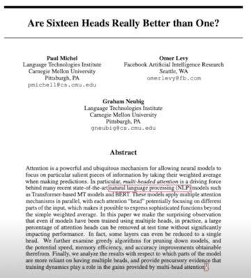
Overview

• Multi-Headed Attention(MHA) allows potentially focusing on different parts of input, which makes it possible to express to sophisticated functions beyond the simple weighted average
• This paper shows
  • Large percentage of attention heads can be removed at test time with small performance degrades
  • Some layers can even be reduced to a single head
  • By simple iterative pruning attention heads, resulting in up to a 17.5% of increase in inference speed
• We mainly focus on findings and experiment on BERT

Are All Attention Heads Important?

• Compute the difference in performance when all heads except one are removed, within a single layer

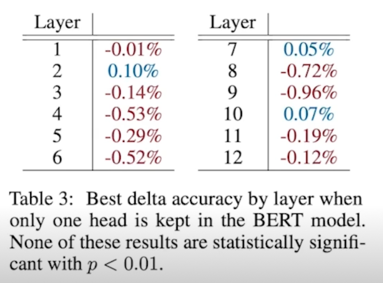
• Authors found that, for most layers, one head is indeed sufficient at test time(these layers can be reduced to single-headed attention)
• However, some layers do require MHA
  • (e.g., last layer in the encoder-decoder attention of NMT)
• In a few layers(2, 3, and 10), it is possible to retain the same level of performance with only one head

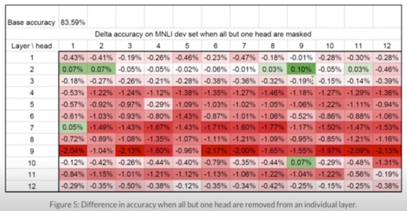
8, 9번에서 성능이 상대적으로 크게 떨어지지만 1~2%도 안되는 성능저하가 일어나서 별 차이가 없더라

• Ablation study on out-of-domain test set to check their generalizability to other datasets (Head selected on: MNLI-matched validation, Tested on: MNLI-mismatched validation)

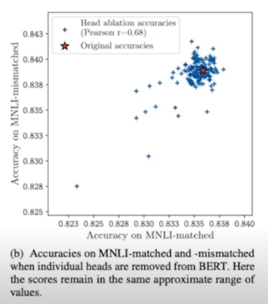
수치적으로 pearson 상관계수가 0.68로 높은 수치를 보이고있고 그래프로 보더라도 MNLI-matched 와 MNLI-mismatched 의 성능차이가 크지 않은 걸 볼 수 있음 중요한 head 는 데이터셋들 간에도 유사성을 보인다

지금까지 특정한 layer 에서 head 를 제거하여 효과를 확인(나머지는 유지), 여러 layer 에 대한 여러 head 를 제거했을 때는 어떤 현상이 발생하는가? (Compounding effect of pruning heads across the model)

Iterative Pruning of Attention Heads

• Sort all the attention heads in the model according to a proxy importance score, and then remove the heads one by one
• ($\xi_h$: mask variables, O: masked(removed), 1: unmasked, $X$: data distribution)

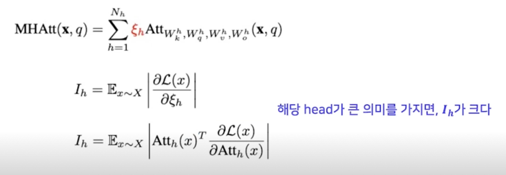
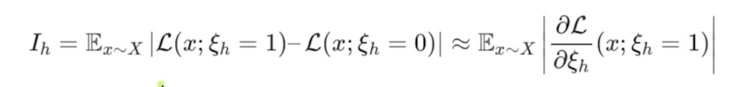
masked variable 이 바뀔때의 loss 의 변화 1 $\rightarrow$ 0 으로 바뀌었을 때 특정 attention 에 3번 head 가 있다가 없어졌다라고 했을 때 loss 의 변화 그러한 변화를 모든 데이터에 대해서 평균을 냄

그래서 얘가 크면 그만큼 없어짐으로 인해서 영향이 크다라는 거니까 그걸 importance score 로 보겠다

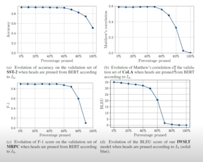
• e.g.) 20% pruning $\rightarrow$ 12 x 12 = 144 heads 중 $I_h$ 가 작은 20%($\approx$ 30개) heads 를 제거한다

• It is possible to reduce the number of heads by up to 60% small loss in performance (for BERT model)

Effect of Pruning of Efficiency

• Pruning 50% of model’s heads speeds up inference by up to 17.5%(for higher batch sizes)

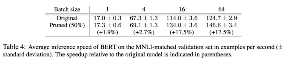
배치사이즈가 작을 땐 효과가 크지 않은데 16개 이상이 되면 16배 정도로 향상

2.1 Pruning; unstructured

Movement Pruning: Adaptive Sparsity by Fine-Tuning(NeurIPS 2019)

Overview

• Magnitude pruning is less effective in the transfer learning regime that has become standard for the SOTA NLP applications
• Why?; Transfer learning, weight values are mostly predetermined by the original model, and are only fine tuned
• Suggests movement pruning, approaches that consider the changes in weights during fine-tuning
• In highly sparse regimes(less than 15% of remaining weights), significantly improves over magnitude pruning
• Reach 95% of the original BERT performance with only 5% of the encoder’s weight on MNLI, and SQuAD v1.1

Magnitude pruning 이 transfer learning 에서는 효과적이지 않음 잘 안됨

왜? fine tuning 시에 weight 의 값의 변화가 크지 않음

original task 에서 값이 컸던 weight 들이 유의미한걸 가진다고 한다면 transfer learning 을 했을 때 실제로 유의미하지 않더라도 점점 줄어드는 방향 이었음에도 그냥 걔가 애초에 값이 컸다는 이유로 pruning 이 안되는 경우가 있다는 것임

그래서 movement pruning 을 제안함

fine tuning 과정에서 weight 가 점점 커지는 방향이냐를 보는 것임

이게 더 효과적임

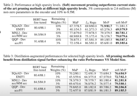
sparse 가 큰 환경에서 weight 를 15%만 남겨놓고 다 날려버림 85% 를 0으로 만들었을 때 magnitude pruning 보다 훨씬 더 좋은 성능을 보임

encoder weight 의 5% 만을 가지고서 95% performance 를 달성했다고 설명

생각의 흐름

• Transfer learning 에서 Weight 의 변화는 그리 크지 않음
• 값이 큰 Weight 은 그대로 값이 큼(Weight 값은 많이 변하지 않음)
• Original model 에서의 큰 Weight 은 Original task 에서 중요한 의미를 갖는 Weight 일 가능성이 큼 <-> Fine-tuned model 에서 큰 Wweight 은 Target task 에서 중요하지 않은 Weight 일 수도 있음
  • (애초에 컸고, 많이 안변하니까…!)
• Magnitude Pruning 에서는 Original task 에서만 중요했던 Weight 들이 살아남을 수 있음

$\rightarrow$ Movement Pruning Transfer Learning 과정에서, Weight 의 움직임을 누적해가며 Pruning 할 Weight 을 결정하자

Background: Score-Based Pruning(Unstructured pruning formulation)

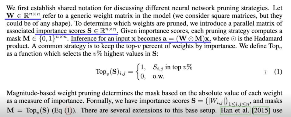
Weight 가 크면 살아남고 작으면 0이 됨

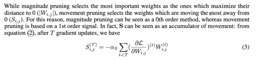
Method Interpretation

• Magnitude pruning can be seen as utilizing $0^{th}$ order information(fixed value) of the running model
• Movement pruning utilizes importance derived from $1^{st}$ order information
• Intuitively, instead of selecting weights that are far from zero(magnitude), retain connections that are moving away from zero during training process

애초에 0에서 멀리 있는 애들을 보는게 아니라 0에서 점점 멀어지는 애들을 볼거다 라는 아이디어

Method Interpretation; Movement Pruning 의 score 유도

• Masks are computed using the $M = Top_v(S)$
• Learn both weights $W$, and importance scores $S$ during training(fine-tuning)
• Forward pass, we compute all $i, a_i = \sum_{k=1}^{n} W_{i,k}M_{i,k}x_k$
• Forward 과정에서, Top 에 속하지 못한 나머지는 masking 이 0이 되어 gradient 값이 없으므로, straight-through estimator(Quantization function 의 back propagation 에서 자주 사용되는 technique)를 통하여, gradient 를 계산
• 단순히, gradient 가 “straight-through” 하게 $S$ 로 전달($M$ $\rightarrow$ $S$)
• $S$ 의 변화에 따른 Loss 의 변화(gradient of the loss w.r.t $S$)는 아래와 같이 정리

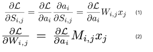
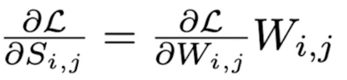
• By combining it (2)(gradient derivation) into (1), we have

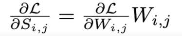
Score 의 변화에 따른 Loss 의 변화는 Loss function 의 Weight 에 대한 Gradient 와 Weight 의 곱과 같다

Method Interpretation; Movement Pruning 의 score 해석

• Gradient descent 를 생각해 볼 때($w = w - \alpha \frac{\partial L}{\partial w}$)
• $W_{i,j} > 0, \frac{\partial L}{W_{i,j}} < 0$ 이면, $W_{i,j}$ 는 증가하는 방향(이미 양수에서 더 커짐)
• $W_{i,j} < 0, \frac{\partial L}{W_{i,j}} > 0$ 이면, $W_{i,j}$ 는 감소하는 방향(이미 음수에서 더 작아짐)
• 즉, $\frac{\partial L}{\partial S_{i,j}} < 0$ 의 경우의 수 두가지에 대해서 모두 $W_{i,j}$ 의 Magnitude 가 커지는 방향

$\rightarrow$ $W_{i,j}$ 가 0에서 멀어지는 것 $\rightarrow$ $\frac{\partial L}{\partial S_{i,j}} < 0$ $\rightarrow$ $S_{i,j}$ 가 커지는 것($S_{i,j} = S_{i,j} - \alpha \frac{\partial L}{\partial S_{i,j}}$)

$W_{i,j}$ 가 0에서 멀어질수록, $S_{i,j}$ 가 커진다 $\rightarrow$ Movement Pruning

Method Interpretation; Movement Pruning 의 score figure

• $W$ 가 0에서 멀어진다 $\rightarrow$ $S$ 가 커진다

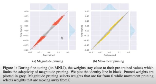
Score 는 Weight 가 fine tuning 되면서 함께 학습

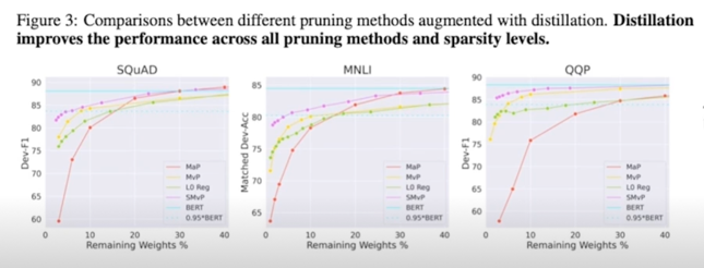
Experiment

• MaP: Magnitude Pruning, MvP: Movement Pruning, SMvP: Soft Movement Pruning
• 정도가 작은 pruning 에 대해서는 다른 기법들이 우세, pruning 의 정도가 커질수록 효과성 증대

Experiment with KD

• KD 가 접목될 경우, SMvP, MvP 의 성능은 눈에 띄게 향상됨 (정도가 작은 Pruning 에 대해서도 성능 향상)

2.1 Pruning; 추천 논문

Encoder 의 각 위치별로 어떤 knowledge 를 가지고 있는가? (1)

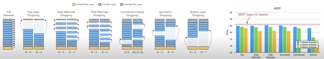
• On the Effect of Dropping Layers of Pre-trained Transformer Models
  (https://arxiv.org/pdf/2004.03844.pdf)
  Pretrained information(general linguistic knowledge(semantics, syntactic 정보))는 input 에 가까운 encoder 들에 저장되어있고, head 에 가까운 부분들은 task specific 한 정보를 저장, pretraining 모델에서 head 쪽 layer 를 없애도 fine-tuning 시의 성능이 크게 떨어지지 않는다.

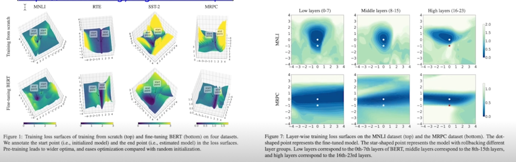
Pretraining-fuin-tuning paradigm 이 왜 성능, generalization capability 가 더 좋은가?

• Visualizing and Understanding the Effectiveness of BERT
  (https://aclanthology.org/D19-1424.pdf)

Structured/Unstructured

• Structured
  • pros: 모델 사이즈 감소, 속도 향상
  • cons: 성능 드랍
• Unstructured
  • pros: 모델 사이즈 감소, 적은 성능 드랍
  • cons: 속도 향상 X (별도 처리가 없는 경우)

2.2 Weight Factorization & Weight Sharing

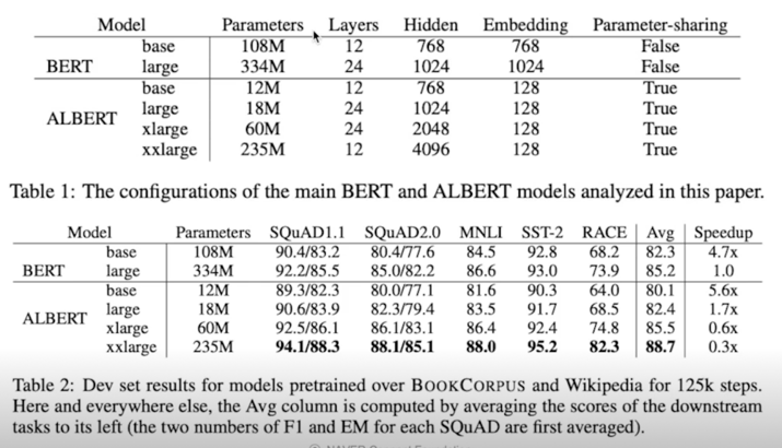
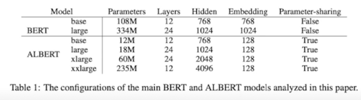
ALBERT: A Lite BERT for Self-supervised Learning of Language Representations(ICLR 2020)

Overview

• Larger network is of crucial importance for achieving the SOTA performance
• Common practice is to pre-train large models and distill them down to smaller ones
• But, Scaling the model faces,
  • 1)Memory Limitations of hardward
  • 2)Communication overhead from distributed training

$\rightarrow$ Suggests, 1) Cross-layer parameter sharing // Parameter 수 감소(1) 2) Next Sentence Prediction $\rightarrow$ Sentence Order Prediction // 성능 향상 3) Factored Embedding Parameterization // Parameter 수 감소(2)

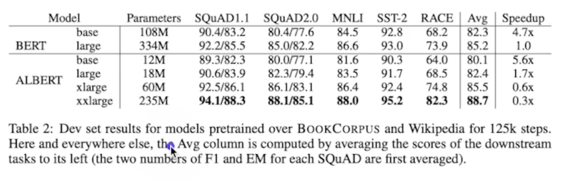
Result in,

• 18x fewer params(BERT-large 유사 성능)
• 1.7x faster training

[Note]

ALBERT never intended to make model smaller, It intended to scale up the model by making model efficiently

(모델을 더 효율적으로 만들어서, 더 큰($\approx$ 더 좋은) 모델을 쓰자!)

Cross-layer parameter sharing

• Parameter sharing to improve parameter efficiency
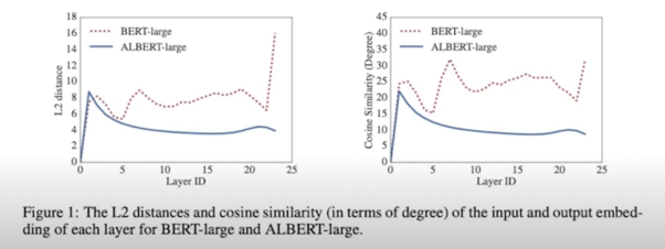
• Fig1, L2 dist, cos-similarity of the input and output embeddings
  • Weight-sharing has an effect on stabilizing network params
  • (Q) Doesn’t this mean as the layer goes deeper, it doesn’t mean much as feature extraction?

• Which one should we share? (e.g., only FFN?, only Attention?)
  Default for ALBERT is all params across layers!
• Guess authors focused more on efficiency of params

Sentence Ordering Objectives

• Conjecture that the Next Sentence Prediction(NSP) is too easy as a task, compared to Masked Language Modeling(MLM)
  • NLP is intended to learn topic prediction, coherence prediction But overlaps with MLM loss
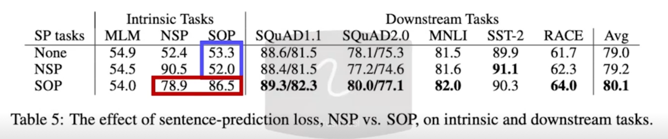
• Sentence Order Prediction(SOP) focuses more on inter-sentence coherence

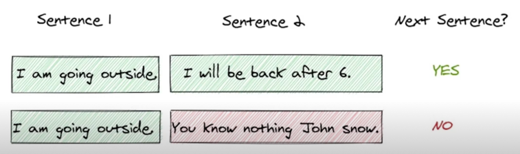
• NSP loss brings no discriminative power to the SOP task
• SOP loss does solve the NSP task as well as SOP task
• SOP loss appears to consistently improve downstream task performance

Factorized Embedding Parameterization

• WordPiece embeddings($E$) are meant to learn context-independent representations
• Hedden layer embeddings($H$) are meant to learn context-dependent representations
• The power of BERT-like representations comes from the use of context to provides the signal for learning such context-dependent representations

“E 와 H 는 BERT 에서 dimension 이 같습니다”

$\rightarrow$ BERT 는 context-dependent representations 의 학습에 효과적인 구조,

왜 BERT layer 가 context-independent representations 인 WordPiece embeddings 에 묶여야 할까?

+ Vocab size($V$)는 일반적으로 매우 큼(30,000 dim)

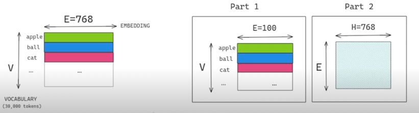
$\rightarrow$ Untying the WordPiece embedding size $E$ from the hidden layer size $H$

• Untying dimensions by using decomposition
• Reduces params $O(V \times H)$ to $O(V \times Ee + E \times H)$
• e.g.) V=30,000, H=768, E=100
  WordPiece Embedding: 30,000 x 768 $\approx$ 23M
  By factorization: 30,000 x 100 + 100 x 768 $\approx$ 3M + 0.07M = 3.07M

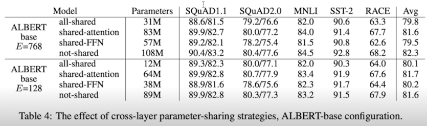
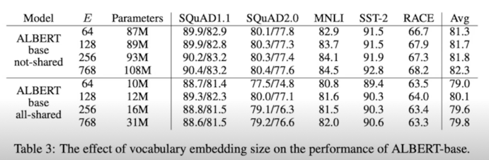
• Effect of changing the vocab embedding size($E$)
• Not-shared seems larger embedding give better performance,(not by much) while all-shared shows $E = 128$ to be the best

Experiment

Comments

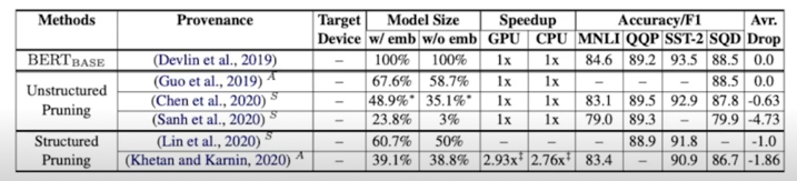
• Parameters written in Table 2, only means “unique” parameters
  $\rightarrow$ We need to calculate large model’s weights(for forward), gradients(for backprop)
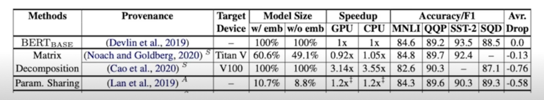
  $\rightarrow$ Note, actual speed up is around 1.2x, with 10.7% of param size(according to [1])

• (일반적인) Matrix decomposition
  • pros: 모델 사이즈 감소, 적은 성능 감소, 속도 향상(주로 cpu)
  • cons: 속도 변화 미미(GPU)
    • 실제로 연산 횟수는 줄어드는데 layer 가 늘어남 그러다보니 병렬처리하는데 있어서 bottleneck 이 생겨서 GPU 에서는 파라미터 줄어드는 대비해서 속도향상이 크지 않음
• Param(Weight) sharing
  • pros: 모델 사이즈 감소, 학습 관련 이점
  • cons: 적은 속도 개선